Article

 

Investigation of Nano-Keyhole Cooling Evolution Using Boubaker Polynomials Expansion Scheme (BPES)

 

M. Dada 1, Olufemi Folorunsho Moses 2*, O. B. Awojoyogbe 1, K. Boubaker 2, K. Isah 1

 

1 Department of Physics, Federal University of Technology, Minna, Niger-State , Nigeria.

2 ESSTT/ 63 Rue Sidi Jabeur 5100 Mahdia, Tunisia. 2*P.O. Box 9352, GDP. Marina Lagos-State, Nigeria.

 

* Corresponding author. Email: boubaker_karem@yahoo.com

 

Citation: M. Dada, et al., Investigation of Nano-Keyhole Cooling Evolution Using Boubaker Polynomials Expansion Scheme (BPES). Nano Biomed. Eng., 2010, 2(1), 8-14.

DOI: 10.5101/nbe.v2i1.p8-14.

 

Abstract

This study proposes an analytical expression for temperature evolution inside a nano-keyhole modeled device. Several assumptions have been taken into account. The validity of the model has been tested through compatibility with experiment and Newtonian cooling laws.

 

Keywords: Keyhole, Heat equation, Newtonian cooling, Boubaker polynomials.

 

1        Introduction

In recent years, numerical modeling has become a realistic method in many applied physics fields [1-5] as for the prediction of weld geometries and time de-pendent evolution. A schematic illustration of the ge-ometrical features of the keyhole weld is provided in Figure(1).In this model tree main assumption are taken into account:

 √The keyhole wall temperature corresponds to the metal boiling point.

√The exciting beam thermal and optical profiles are coherent..

√The absorption coefficient is constant on keyhole wall.

As shown in Fig1, the y-direction is the direction of motion of the laser beam (welding direction) and since according to the nano-keyhole approximation model, the nano-keyhole vertical edges temperature is equal to the boiling point of the material, it would be expected that heat transfer is in the x-direction. Under these assumptions, the one-dimensional diffusion, or heat equation for this experimental setup would be derived as follows.

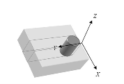
 Figure 1. Nano-keyhole model geometrical features

 

2        Temperature Dimensionless Expression Derivation Materials

Let Tl (x, t) represent the dimensionless temperature of a metal bar at a point x at time t. The first step is the derivation of a continuity equation for the heat flow in the bar shown above. If the bar has a cross sec- tional area A, so that the infinitesimal volume of the bar between x and x x is Ax . The quantity of heat contained  in  this  volume  is cpTl Ax , with c p the specific heat, the mass per unit volume; their product has dimensions c p ML1T 21 . In a time interval dt this heat changes by an amount due to the change in temperature. This change in the heat must come from laser beam extraor- dinary excitation of the atoms of the bar, and is the result of a flux of heat q(x,t) (released by the atoms that have been excited by the laser beam) through the area A (q is the heat flowing through a unit area per unit time). Into the left side of the volume an amount of heat qAdt flows in a time dt; on the right hand side of the volume a quantity: , schematic illustration of the geometrical features of the nanokeyhole weld flows out in a time dt, so that the net accumulation of heat in the volume is . Equating the two expressions for the rate of change of the heat in the volume Ax  we find: 

which is the equation of continuity [6]. It is a mathematical expression of the conservation of heat in the infinitesimal volume Ax. We supplement this with a phenomenological law of heat conduction, known as Fourier's law: the heat flux is proportional to the negative of the local temperature gradient (heat flows from a hot region to a cold region):

with the thermal conductivity of the metal bar. The thermal conductivity is usually measured in units of and has dimensions MLT 31 . Combining Eq. (1) and Eq. (2), we obtain the diffusion equation (often called the heat equation)

where is the thermal diffusivity of the bar; it has dimensions as it should. Eq. (3) is the diffusive equation for heat. It usually results from combining a continuity equation with an empirical law which expresses a current or flux in terms of some lo-cal gradient. Suppose that the bar is very long, so that we can consider the idealized case of an infinite bar. At initial time t = 0, we add an amount of heat H (with dimen-sions [H]=ML2T-2) at some point of the slab (H is the heat energy equivalent of the laser beam power absorbed by the slab during welding; it is as a result of the excitation of the slab atoms), which we will arbi-trarily call x = 0. The heat is conserved at all times, so that:

However, the material to be welded is not infinite in length and provided that heat energy is still conserved within the finite spatial limit N, in consequence Eq. (4) alters to:

The temperature depends upon x, t, and the dif-fusivity D, From Eq. (4), it also depends upon the ini-tial conditions through the combination Dimensional analysis yields a solution to the dif-fusion equation of the form:

By using the chain rule to calculate various derivatives of , we have:

Then, by substituting Eq. (7) into the diffusion equation Eq. (3), and canceling various factors, we obtain a differential equation for :

Dimensional analysis has reduced the problem from the solution of a partial differential equation in two variables to the solution of an ordinary differential equation in one variable. The normalization condition, Eq. (4), becomes in these variables:

Eq. (8) is an exact differential, and it follows that

which we can integrate once to obtain

However, since any physically reasonable solution would have both

 (since there is no way the thermal vibration could get to such point and hence the temperature there would be constant with respect to the immediate environment), the integration constant must be zero. We now need to solve a first order differential equation, which we do by dividing Eq. (11) gives:

where C a constant. To determine C, we use the normalization condition, Eq. (9):

where the integral (known as a Gaussian integral) can be found in integral tables. If we have a very big slab to weld such that the axis through which the laser beam would pass is quite small compared to the over-all dimension of the slab, the expression of Eq. (13) would hold, at least approximately. Therefore:

This is the complete solution for the temperature distribution in a within the one-dimensional bar due to a point source of heat (Figure 2).

 

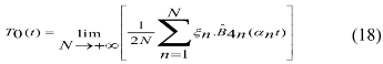
3        Maximum Temperature Rise T0expression Derivation

3.1 Coulomb approximation

By analogy with Coulomb approximation [7], the maximum central temperature T0 rise could be determined:

where b is the radius of the cylindrical targeted zone, receiving a uniformly distributed power P (Figure3), its surface constant temperature rise is expressed by (15). Now, provided that T0 is the the change (rise) in the surface temperature just immediately after the beam passes the nano-keyhole and since Tl is the temperature measured at any given point (we take Tl as our final temperature for this particular situation) we may write that:

T0=T1-T∞

Where we have assumed that T∞ is our initial temperature of the slab. In the absence of work done, a change in internal energy per unit volume in the material, ΔH, is propor-tional to the surface temperature rise. That is:

Where cp is the specific heat capacity, T0=ΔT1=T1-T∞  and ρ is the mass density of the material. Now since the rate of change of the heat energy H is the result of the power delivered per unit volume of the slab (the power is responsible for increasing the internal energy), we may then write that:

Since only T0 depends on time. Since the diffusivity is given as and using Eq. (15), we have:

 

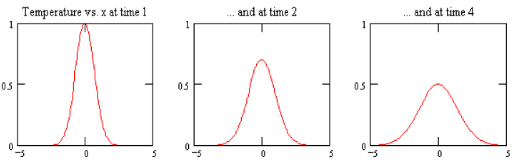
Figure 2. Solution for temperature distribution

 

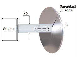
Figure 3. Coulomb approximation scheme

 

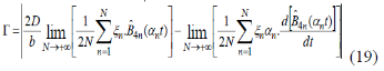
3.2 Boubaker polynomials expansion scheme BPES

Equation (17), it solved using the Boubaker polynomials expansion scheme BPES [8-18]. For this purpose, the t-dependent component of T0 is expressed as:

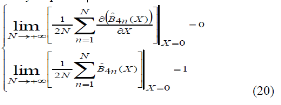
where n are the minimal positive roots of the 4n- Boubaker [9-17] polynomials , N is an integer parameter, and n are coefficients to be found. According to the BPES [12-16] principles, and the re-formulation of Eq. (17), the coefficients minimize the real function : 

Thanks to the properties of the 4n-Boubaker poly-nomials Eq.(20), the main initial conditions are intrinsically respected.

A plot of the obtained expression of T0 against t for Carbon steel slab (D=1.172x10-5m2/s), is given in Figure 4. Figure 5 show the dependence of the yielded solution versus the radius b.  

 

4        Newtonian Cooling

A bigger challenge is actually to see if the Newton’s law of cooling could be used to explain the cooling of the slab after the application of the laser beam. Newton's law of cooling states that the rate of heat loss of a body is proportional to the difference in temperatures between the body and its surroundings, or environment. The law is:

Q = Thermal energy transfer in joules, h= Heat transfer coefficient, A = Surface area of the slab, T0 = Temperature of the object's surface, T∞ = Temperature of the environment. As this form of heat loss principle is sometimes not very precise; an accurate formulation may require analysis of heat flow, based on the (transient) heat transfer equation in a nonhomogeneous, or else poorly conductive, medium. The following simplification may be applied so long as it is permitted by the Biot number (which relates surface conductance to interior thermal conductivity in a body). If this ratio permits, it shows that the body has relatively high internal conductivity, such that (to good approximation) the entire body is at same uniform temperature as it is cooled from the outside, by the environment. If has relatively high internal conductivity, then it is easy to derive from these conditions the behavior of exponential decay of temperature of a body. In such cases, the entire slab is treated as lumped capacitance heat reservoir, with total heat content which is proportional to simple total heat capacity , and the temperature of the body. If T(t) is the temperature of such a body at time t, and Tis thetemperature of the environment around the body, then

Where r is a positive constant characteristic of the slab, which must be in units of 1/time, and is therefore sometimes expressed in terms of a time constant: r = 1/t0. The solution of this differential equation, by standard methods of integration and substitution of boundary conditions, gives:

Here, Tl(t) is the temperature at time t, and Tl(0) is the initial temperature at zero time, or t = 0. If:Tl(t) is defined as: where is the initial temperature difference at time 0, then the Newtonian solution is written as:  

Since the emphasis here is on cooling, we may assume that our investigation process starts immediately after the source of increased temperature has been removed. Hence, Tl(0) is the highest temperature achieved after which surface temperature begin to drop (cooling). The behaviour of Tl(t) is shown in Figure (6). )  (Tl(0) is taken to be 640℃ while T∞is taken to be 27℃. )

Figure 6. A plot of Tl (or T) against time and the time constant

 

5        Conclusions

In this work, theoretical investigations have been per-formed in order to predict temperature distribution evolution in a particular device model: The nano-keyhole model [19-24]. The use of the Colombian ap-proximation 7], Newtonian laws along with the already established Boubaker polynomials expansion scheme BPES [8-18], allowed monitoring temperature dynam-ical profiles. The yielded profiles could be compared successfully compared to those published by R. Rai et al. [25], H. Al-Kazzaz et al. [26], P. Solana et al. [27], and C. S. Wu et al. [28].

 

References

1. Suh HJ, Lee KJ, Curr. Appl. Phys. 9 (2009) 985-988 doi:10.1016/j.cap.2008.10.004
2. Zahangir Kabir M, Yunus M, Kasap SO, Tousignant O, Mani H, Gauthier P, Curr. Appl. Phys. 6 (2006) 393-398 doi:10.1016/j.cap.2005.11.026
3. Essimbi BZ, Jäger D, Curr. Appl. Phys. 6 (2005) 567-571 doi:10.1016/j.cap.2004.06.025
4. 4 Yoon SH, Jung JS, Lee CS, Yoon IT, Won T, Curr. Appl. Phys. 2 (2002) 253-255 doi:10.1016/S1567-1739(02)0 0102-5
5. Chang DH, Jeong SH, Hong BG, Chung KS, Kim GH, Lee JS, Curr. Appl. Phys. 6 (2001)497-503 doi:10.1016/S1567-1739(01)00062-1
6. De P, Current Applied Physics, Curr. Appl. Phys. 76 (2007) 274-280 doi:10.1016/j.cap.2006.08.001
7. Kühn JH, Penin AA, Pivovarov AA, Nuclear Phys. 534 (1998) 356-370 doi:10.1016/S0550-3213(98)00607-5
8. Ghanouchi J, Labiadh H, Boubaker K, Int. J.of Heat & Tech., in press.
9. Awojoyogbe OB, Boubaker K, Curr. Appl. Phys. 9 (2009)278-283 doi:10.1016/j.cap.2008.01.019
10. Boubaker K.Trends in Applied Science Research, 2(2007) 540-544 doi:10.3923/tasr.2007.540.544
11. Labiadh H. Journal of Differential Equations and Control Processes, 2 (2007) 117-133
12. Lazzez S, Ben KB,Mahmoud, Abroug S, Saadallah F, Amlouk M. Curr. Appl. Phys. 9 (2009) 1129-1133 doi:10.1016/j.cap.2008.12.010
13. Fridjine S, Ben KB, Mahmoud, Amlouk M, Bouhafs M. J. of Alloys and Comp., 479, (2009) 457-461 doi:10.1016/j.jallcom.2008.12.139
14. Ben KB, Mahmoud, Amlouk M. Materials Letters, 63 (2009) 991-994 doi:10.1016/j.matlet.2009.01.063
15. Karem M, Ben Mahmoud. Cryogenics 49 (2009) 217-220 doi:10.1016/j.cryogenics.2009.01.007
16. Zhao TG, Ben BK, Mahmoud, Toumi MA, Faromika OP, Dada m, Awojoyogbe OB, Magnuson J, Lin F, Differential Eq J. Control Processes, 1 (2009)7-19.
17. Zhao TG, Wang YX, Ben BK, Mahmoud. Int. J. of Math. and Comp. 1(2008)13-16.
18. Oyodum OD, Awojoyogbe OB, Dada M, Ben KB, Mahmoud, Magnuson J. Eur. Phys. J. Appl. Phys. 46 (2009) 21201 doi:10.1051/epjap/2009036
19. Kaplan A. A model of deep penetration laser welding based on calculation of the keyhole profile, J. Phys. D: Appl. Phys. 27 (1994) 1805–1814. doi:10.1088/0022-3727/27/9/002
20. Lampa C, Kaplan AFH, Powell J, Magnusson C, An ana-lytical thermodynamic model of laser welding, J. Phys. D: Appl. Phys. 30 (9) (1997) 1293–1299.doi:10.1 088/0022-3727/30/9/004
21. Jin X, Li L, Zhang Y. A study on fresnel absorption and reflections in the keyhole in deep penetration laser weld-ing, J. Phys. D: Appl. Phys. 35 (2002) 2304–2310. doi:10.1088/0022-3727/35/18/312
22. Dowden J, Postacioglu N, Davis M, Kapadia P. A key-hole model in penetration welding with a laser, Journal of physics. D, Applied physics 20 (1987) 36-44 doi:10.1088/0022-3727/20/1/006
23. Semak VV, Bragg WD, Damkroger B, Kempka S. Tran-sient model for the keyhole during laser welding , J. Phys. D: Appl. Phys. 32 (1999) 61-64 doi:10.1088/0022-3727/32/15/103
24. Ki H, Mazumder J, Mohanty PS. Modeling of laser key-hole welding: Part II. simulation of keyhole evolution, velocity, temperature profile, and experimental verifica-tion, Metallurgical and Materials Transactions A, 33(2002) 1831-1842 doi:10.1007/s116 61-002-0191-5
25. Rai R, Kelly SM, Martukanitz RP, DebRoy T, A Con-vective Heat-Transfer Model for Partial and Full Pene-tration Keyhole Mode Laser Welding of a Structural Steel, Metallurgical and Materials Transactions A, 39 (2008) 98-112 doi:10.1007/s11661-007-9400-6
26. Al-Kazzaz H, Medraj , Caoand X, Jahazi M. Nd:YAG laser welding of aerospace grade ZE41A magnesium al-loy:Modeling and experimental investigations,Materials Chemistry and Physics 109 (2008) 61–76
27. Solana P, Negro G. A study of the effect of multiple reflections on the shape of the keyhole of the keyhole in the laser processing of materials, J. Phys. D: Appl. Phys. 30 (1997) 3216–3222.doi:10.1088/0022-3727/30/23/006
28. Wu CS, Wang HG, Zhang YM. A new heat source mod-el for keyhole plasma arc welding in FEM analysis of the temperature profile, Welding journal 85 (2006) 284-289.

 

Received 26 January, 2010; accepted 18 February, 2010; published online 5 March, 2010.

 

Copyright: (c) 2010 M. Dada et al. This is an open-access arti-cle distributed under the terms of the Creative Commons Attribution License, which permits unrestricted use, distribu-tion, and reproduction in any medium, provided the original author and source are credited.